|
|
|
 |
General
The Discrete Direct Fourier Transform and the Discrete Inverse Fourier Transform (hereafter denoted by FT and iFT respectively) are used to change the representation of a function from one vector space to another isomorphic vector space. The Fourier Transforms connect the Discrete Time-Amplitude vector space (where each vector is the value of a signal at a given discrete time moment) with the Discrete Frequency-Amplitude vector space (where each vector is the value of one spectral component for a given discrete frequency). The FT makes the Transformation from the Time-Amplitude space to the Frequency-Amplitude space, and the iFT makes the Transformation from the Frequency-Amplitude space to the Time-Amplitude space.
The FFT (Fast Fourier Transform) and iFFT (Inverse Fast Fourier Transform) algorithms were designed to increase the speed of the FT and iFT calculation; they are applicable to input vectors with a number of samples N a power of two N=2^m.
Note
The term "vector" as used throughout this document generally represents
an array of complex numeric values and, unless otherwise specified, it
is not related to the term "vector" used in the vector space theory.
The X[k] FT vector elements are calculated according to the following
formula from the x[] input vector:
X[k] = FT(x[]) = C1 Sum(x[n]exp(-2 i PI k/N n)), n in [0,
N-1]
The x[n] iFT vector elements are calculated according to the following
formula from the X[] input vector:
x[n] = iFT(X[]) = C2 Sum(X[k]exp(2 i PI n/N k)), k in [0,
N-1]
The relation linking the FT and iFT is:
iFT(FT(x[])) = x[], where x[] is a time-domain vector
or, equivalently:
FT(iFT(X[])) = X[], where X[] is a frequency-domain vector
These relations imply the following condition for the two constants
C1 and C2:
C1 C2 = 1
In order to further define the values of C1 and C2, a
physical-interpretation-related condition has to be stated: it will be
assumed that, given a unitary transfer function in the frequency domain
H1[]=1[] and its corresponding time-domain representation
h1[]=Kronecker0[], a signal x[] convoluted ("filtered") with h1[] will
equal the original signal x[]. Given that h1[] = iFT(H1[]) (and
implicitly also FT(h1[]) = H1[]) the following formulae result:
C1 = 1;
C2 = 1/N;
The FT and iFT definitions also imply the two transforms are
periodic functions with period N (each the real part, the imaginary
part, and the modulus have the period N):
x[n+N] = x[n] (fig. 6a shows the x[] modulus periodicity
for a causal low-pass filter)
X[k+N] = X[k] (fig. 6b shows the X[] modulus periodicity
for a causal low-pass filter)
The following set of two-way implications exists between the Real
and Imaginary parts of the transforms, for a Real "input" function (see
Fig.4a, Fig.4b, and Fig.5c, Fig.5d in the FIR
presentation section):
If and only if Im(x[n]) = 0 for any n in the definition domain
then the following relations hold true:
Re(X[-k]) = Re(X[k]),
Im(X[-k]) = -Im(X[k]),
The complementary set of relations (obtained by X[] <=> x[]) also
holds true:
If and only if Im(X[n]) = 0 for any n in the definition domain
then the following relations hold true:
Re(x[-k]) = Re(x[k]),
Im(x[-k]) = -Im(x[k]),
The following one-way implications can also be derived from the
above:
If Im(x[n]) = 0 for any n in the definition domain then the
following relations hold true:
Abs(x[-k]) = Abs(x[k]),
and
If Im(X[n]) = 0 for any n in the definition domain then the
following relations hold true:
Abs(X[-k]) = Abs(X[k]),
The proof for the results mentioned in this paragraph is beyond the scope of this presentation.
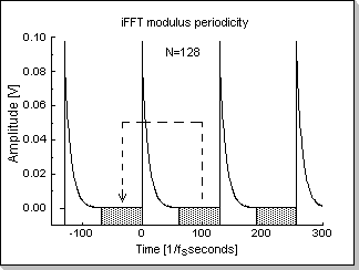 Fig.6a |
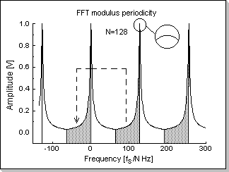 Fig.6b |
The Definition Domains for the FFT and iFFT functions
The standard FFT/iFFT algorithms calculate the Discrete Fourier
Transform X[k] with k in [0, N-1] for a signal x[n] with n in [0, N-1].
However, because the FT(x[]) and iFT(X[]) are periodic functions with
period N, any contiguous N-point definition domain can be specified for
both the X[] and x[] vectors:
The vector X[k] with k in [-N/2, N/2-1] is an equivalent representation
of X[k] with k in [0, N-1] (i.e. the X[N/2] to X[N-1] sub-domain
translates into the X[-N/2] to X[-1] sub-domain)
The vector x[n] with n in [-N/2, N/2-1] is an equivalent representation
of x[n] with n in [0, N-1] (i.e. the x[N/2] to x[N-1] sub-domain
translates into the x[-N/2] to x[-1] sub-domain)
Remark
In order to calculate the FFT/iFFT for a zero-centered domain, the
input data vector has to be permuted first (the negative sub-domain
[-N/2,-1] has to be appended to the positive sub-domain [0, N/2-1] in
order to produce a proper [0,N-1] definition domain for the standard
FFT/iFFT algorithm calculation), and the result vector will also have
to be premuted back (from [0,N-1] to [-N/2, N/2-1]) at the end of the
algorithm (see fig.6a and fig.6b).
The CDSPLib implementation embeds the initial and final domain swapping (that allow zero-centered intervals calculations) in the FFT/iFFT algorithms, thus preventing time-consuming data moves. This way the interface the FFT/iFFT functions present to the user consists of both zero-centered [-N/2, N/2-1] domain vectors (this approach is taken to maintain direct compatibility with the other vectors used throughout most of the CDSPLib library functions), and positive [0, N-1] domain vectors (this may be useful for of-the-shelv algorithms developed for direct interfacing with the standard FFT/iFFT algorithms). The type for the definition domains is a run-time programmable parameter of the FFT/iFFT library functions.
Conditions for the numeric values involved in the FFT and iFFT calculations
The FFT and iFFT algorithms contain multiplication and addition operations, thus being susceptible to generate internal overflows; in order to prevent them, a number of restrictions (conditions) are imposed on the input vector elements' modulus. Following is a discussion of the overflow possibilities in the FFT algorithm.
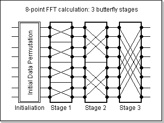 Fig.7a |
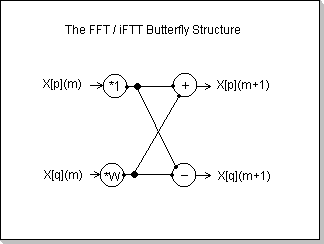 Fig.7b |
The N-point FFT algorithm is based on Log2(N) stages (Fig.7a) of
butterfly structures (Fig.7b). Each stage of the FFT consists of
independent butterfly calculations, where the butterflies in one single
stage do not interfere with each other. Thus, at the output of each
stage, each pair of elements will be the result of the butterfly
calculation formula:
X[p](m+1) = X[p](m) + w X[q](m)
X[q](m+1) = X[p](m) - w X[q](m)
where p and q are the two nodes of the butterfly, m and m+1 are two
consecutive FFT stages, and w is the complex twiddle constant with
Abs(w)=1
The butterflies' nodes are connected in a special way commonly known as
"bit-reverse order".
By considering all x[p] inputs to be Abs(x[p])<1, the above
butterfly formula recursively leads to the conclusion that any element
X[p](m) (in stage m inside an FFT transform calculation) will have the
property Abs(X[p](m))<2^m. In particular, the output elements X[p]
of the FFT transform will all be Abs(X[p])<2^N.
Because the CDSP's calculations are performed in fixed-point format,
range [-1,1), it results that in order to prevent output overflows (and
implicitly any intermediate internal overflows) during the FFT
algorithm, the input vector's absolute values must all be smaller than
1/N: Abs(x[p])<1/N
In the case of the iFFT transform, the multiplication with the 1/N constant can be made at the beginning of the algorithm, i.e. on the input values. Consequently, the input vector's absolute values must all be smaller than 1: Abs(x[p])<1.
To summarize:- in order to prevent any overflow during the FFT calculation, the range of the input vector's absolute values must be (-1/N, 1/N)
- in order to prevent any overflow during the iFFT calculation, the range of the input vector's absolute values must be (-1, 1)
Numeric Precision Enhancement
The FFT/iFFT algorithms allow a numeric precision enhancement method based on the successive stages structure of the calculations. This method can be directly applied to the iFFT algorithm, and indirectly to the FFT.
It can be seen from the iFFT formula that its calculation involves a division of the input values by N, where N is the number of sampling points. However, this operation can be split throughout the m=Log2(N) stages involved in the iFFT: at the beginning of each stage, the intermediary stage input values can be divided by 2. This results in a significantly greater calculation precision than if one would directly divide the input values by N at the beginning of the algorithm, while still preventing any internal overflows. This way calculations will be performed with (b-1)–bit fixed-point numbers instead of (b-Log2(N))–bit fixed point numbers, where b is the CDSP word length (for example, if N=256 and b=16, then this method will increase the internal calculations precision from 8 bits to 15 bits).
Remark
This method of internal calculation (i.e. dividing by 2 at the
beginning of each butterflies stage) can also be used for the direct
FFT. In this case the output results will be numeric values 1/N times
the true FFT result (because the FFT definition does not contain the
division by N). By using this method, the range of the input's absolute
values can be increased to (-1,1) as compared to the (-1/N, 1/N) range
for the "normal" FFT algorithm, while still preventing any internal
overflows. In order to obtain the correct FFT result, the outputs will
have to be multiplied by N.
If another algorithm that involves a division by N is chained at the
end of the FFT, then the successive FFT-output's multiplication with N
and the chained-algorithm's division by N can be skipped, while
maintaining a high, b-Log2(N) -bit, calculations precision.
The FFT/iFFT Implementation
The FFT/iFFT components
The FFT/iFFT module has the following interface elements:
- a variable that holds the number of sampling points N (there will thus be m=Log2(N) stages)
- a flag variable that specifies the type of definition domains for the input and output vectors (zero-centered vs. positive-defined domain)
- a vector that holds the twiddle factors
- a vector that holds the input values at the beginning of the FFT/iFFT, the intermediary values during the calculations, and the result values after the FFT/iFFT algorithm is completed
- a function that fills the twiddle vector with the FFT twiddle factors
- a function that fills the twiddle vector with the iFFT twiddle factors
- a function that performs the initialization (an input data permutation in the input/output vector)
- a function that performs the FFT transform, i.e. with no division constant
- a function that performs the iFFT transform, i.e. including the division by N (as previously described, the division constant N is spread thru the m=Log2(N) stages of calculations)
Remark
The number of stages and the length of the vectors are directly derived
from the number of sampling points.
The FFT/iFFT usage
The FFT and iFFT algorithms are performed on chunks of data; they are not per-sample calculations. In order to compute the transform for an input data vector, the following operations have to be performed:
- the number of sampling points has to be programmed
- the definition domains type has to be programmed
- the FFT or iFFT twiddle factors calculation function has to be called, depending on the desired function
- the input/output vector has to be loaded with the input data
- the FFT/iFFT initialization function has to be called (performing the initial data permutation)
- the FFT or iFFT calculation function has to be called
- the result data in the input/output vector has to be extracted
Example 1
This example shows a real sinus input vector with the imaginary part all zero (Fig.8a) and its corresponding FFT transform (Fig.8b). The only spectral components of the sinewave are f0 and -f0 corresponding to the input signal's frequency.
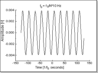 Fig.8a |
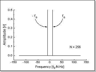 Fig.8b |
Remark
The input signal's amplitude has been chosen smaller than 1/N (in this
case 1/256) in order to prevent frequency-domain overflows; it can be
seen that in this case the sum of the FFT amplitudes for the f0 and f0
components resulted smaller than 1.
Example 2
This example shows a real noisy sinus input with the imaginary part zero (Fig.9a) and its corresponding FFT transform (Fig.9b). The spectrum of the signal contains the f0 and -f0 components, and also relatively small non-zero values along the whole frequency axis corresponding to the input noise.
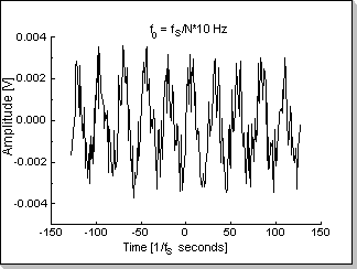 Fig.9a |
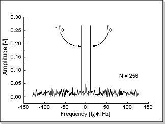 Fig.9b |
Remark
The input signal's amplitude has been chosen smaller than 1/N (in this
case 1/256) in order to prevent frequency-domain overflows.