|
|
|
 |
General
The discrete correlation function, hereafter denoted by R(x1,x2)[],
takes two vectors x1[] and x2[] as arguments and returns a result
vector y[]=R(x1,x2)[]. The y[] result is calculated according to the
following formula:
R(x1,x2)[n] = Sum(x1[m] x2[m-n]), m in (-inf, +inf)
Remark 1
It can be seen from the above formula that the correlation and the
convolution functions are related (see the FIR
filters section):
R(x1,x2)[] = x1 * x2, where x2[i] =
x2[-i] (i.e. x2 denotes x2 with the time scaled reversed)
Remark 2
In the continuous domain, the correlation function is calculated
according to the following formula:
R(x1,x2)(u) = Integral(x1(t) x2(t-u) dt), t in (-inf,
+inf)
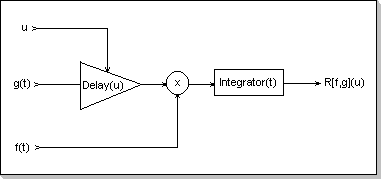
Fig. 16: Time-domain correlator
It can be seen that the correlation function between two sine
functions s1(t) = a1 sin(w1 t + p1) and s2(t) = a2 sin (w2 t + p2) is:
R(s1, s2)(u) = {
   w1 /= w2: Zero(u)
   for w = w1 = w2: a1 a2 cos (w u - (p2-p1))
}
By considering two functions x1(t) and x2(t) as the sum of their spectral components, in the multiplication inside the correlation integral only the spectral components of x1 and x2 that have the same frequency contribute to the integral result (partial results are non-null only for w1 = w2). It can thus be seen that the correlation function is a measure of the resemblance of the two spectra corresponding to x1 and x2, taken on an element by element basis.
Conditions for the input and output vectors' dimensions
As it can be seen from the discrete correlation function definition, the summation is made over the whole (-inf, +inf) interval. Thus, in order to be able to effectively compute a correlation function between two vectors (as a finite number of steps), some restrictions have to be imposed on the vectors' dimensions (i.e. the definition intervals for the two inputs and the output).
Having two x1[] and x2[] input vectors, with the dimension d1 of
x1[] greater than or equal to the dimension d2 of x2[], a (d1-d2)
-sized y[] correlation vector will result.
The following condition for the vectors definition domains can be
derived: for x1[] defined inside [M1, M2-1] and x2[] defined inside
[N1, N2-1], the correlation result y[] will be defined inside [N2-M2,
N1-M1].
Observation
In order to use the same "type" of vector definition domains for both
input and output (i.e. [X, Y-1] instead of [X, Y]), only the [N2-M2,
N1-M1-1] result vector domain will be considered. This also implies
that the x1[M1] sample will not be used during the correlation
calculation (this value only affects the y[N1-M1] output sample).
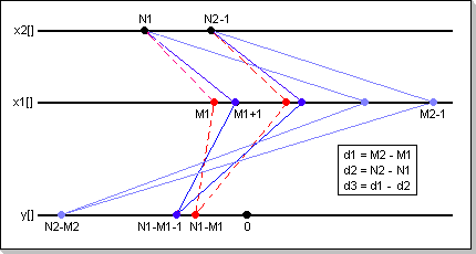
Fig.17: Definition domains for the correlation input and output
Vectors
It can be seen from the correlation formula that the absolute position of the two input vectors is not relevant for the output calculation; only the relative position of the two input vectors affect the result.
Conditions for the numeric values involved in the correlation function calculation
In order to prevent internal overflows, a number of conditions have
to be imposed on the input vectors' values. Given the correlation
formula and the fact that the CDSP operates on fixed point complex
numbers with Abs(p)<1, the general overflow-prevention condition is:
Max(Abs(x1[i])) * Max(Absx2([j])) < 1/d2 for any i
in the x1[] definition domain, and any j in the x2[] definition domain;
here d2 is the dimension of the x2[] vector.
A number of sufficient conditions can be derived from the above
general condition:
- Abs(x1[i]) < 1/d2 for any i in the x1[] definition domain, i.e. the modules of all values in the first input vector (x1[]) have to be smaller than 1/d2
- Abs(x2[i]) < 1/d2 for any i in the x2[] definition domain, i.e. the modules of all values in the second input vector (x2[]) have to be smaller than 1/d2
- Abs(x1[i]) < 1/Sqrt(d2) and Abs(x2[j]) < 1/Sqrt(d2), for any i in the x1[] definition domain and j in the x2[] definition domain, i.e. the modules of all input values in both x1[] and x2[] input vectors have to be smaller than 1/Sqrt(d2)
Remark
It can be seen that the numeric values conditions for the correlation
function are similar to the ones required for the convolution, by
considering the correlation x2[] input vector as the correspondent of
the convolution h[] weights vector (see the FIR
filters section).
The Correlator Implementation
The Correlator Components
The correlation module consists of the following user-accessible components:
- an x1[] input vector used to hold the first correlation argument
- an x2[] input vector used to hold the second correlation argument
- an y[] vector in which the correlation result is calculated
- a six-argument function that defines the definition domains for the vectors (input and output)
- a function that inserts a sample in the first (x1[]) vector (the vector behaves like a FIFO)
- a function that inserts a sample in the second (x2[]) vector (the vector behaves like a FIFO)
- a function that calculates the correlation (fills the output vector with the R(x1,x2) correlation values)
- a function that extracts successive result values from the output vector (for example, if the output vector's definition domain is [R1, R2-1], the first extracted value is y[R1], and the last is y[R2-1]). This function uses an internal iterator to extract the successive values; the iterator is reset by both a specific iterator-reset function, and when performing a new correlation output calculation.
- an output-iterator reset function (mentioned above)
- a function that extracts a value specified by its index from the y[] result vector (for example, for i inside the definition domain of the result vector, the y[i] value will be returned)
- a reset function that clears all buffers and resets the vectors' dimensions to -1 (undefined)
The Correlator Usage
In order to calculate the correlation function between two input vectors, the following procedure has to be applied:
- the "reset" function has to be called;
- the vectors definition domains have to be specified by calling the domain definition function
- the x1[] values have to be input, one at a time, by successive calls to the x1[] sample input function
- the x2[] values have to be input, one at a time, by successive calls to the x2[] sample input function
- the correlation calculation function has to be called, resulting in the y[] vector being filled with the correlation values
- the y[] output values have to be extracted with one of the result-extracting functions (either successively or by specifying the index position). When the entire output vector y[] is needed, the iterative extraction function should be used (it is significantly faster than its positional extraction counterpart)
As previously described, in order to calculate the correlation function of two input vectors for a specific domain, the following relation must hold true between the input and output vectors definition domains:
x1[] : [M1, M2-1]This relation is checked by the function that sets the vectors dimensions, and an error code is returned if the relation does not hold.
x2[] : [N1, M2-1]
y[] : [N2-M2, N1-M1-1]
Example 1
The correlation function between two vectors is calculated by
successively inputting the first vector's values in x1[], the second
vector's values in x2[], and then calling the correlation calculation
function. In this way the correlation function for two impulses can be
calculated.
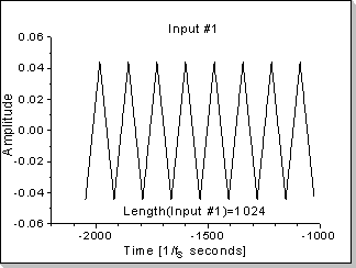 Fig.18a |
|
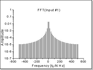 Fig.18b |
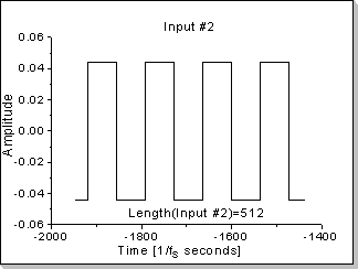 Fig.18c |
|
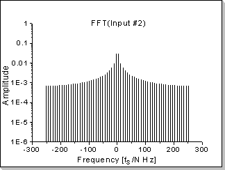 Fig.18d |
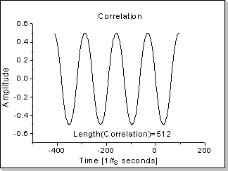 Fig.18e |
|
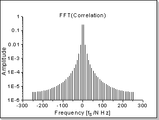 Fig.18f |
Fig.18: Correlation function between two impulses
In this example the correlation function between a triangular waveform-based impulse and a rectangular waveform-based impulse is calculated.
Remark
It can be seen in Fig.18b, Fig.18d, and Fig.18f that the correlation
function's Fourier Transform components are proportional with the
product of the two inputs' Fourier Transforms, taken component by
component (in this example a near-sinewave waveform results, i.e. very
low harmonics that rapidly decrease on the frequency scale).
Example 2
The correlation function between the "most recent" (last) values of an
input data stream and a "reference" vector x2[] can be calculated using
the FIFO functionality of the input vectors: By successively inputting
new values in the x1[] vector and calling the correlation calculation
function, a per-input-sample correlation function can be calculated for
every new input sample.
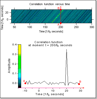
Fig.19: Recognizing a pattern in an input data stream
In this example the correlation function between a long input data
stream and a relatively short reference signal (200 samples long) is
calculated. The input data stream has been chosen to be a highly random
signal, while for the reference signal a portion of the input data
stream itself has been used (this choice has been made to assure that
the correlation function will be sharp enough to be easily visible).
Fig.19 shows the evolution in time of the correlation function,
calculated on a 40-sample domain (the correlation of the last 240
samples of the input data stream and the 200-sample reference signal is
calculated every time a new sample is received from the input data
stream).
The top side of Fig.19 shows the correlation function calculated at
different moments between t=40/fs and t=300/fs seconds (fs is the
sampling frequency); the correlation function at a given moment
(calculated on the [-10,+29] interval) is shown using a color scale
representation.
The bottom side of Fig.19 shows the correlation function calculated at
moment t = 200/fs; the correspondence between the color scale used in
the top side of Fig.19 and the correlation function amplitude is also
shown.
Example 3
The correlation function between the "most recent" (last) values of two
input signals can be calculated using the FIFO functionality of the
input vectors: By successively inputting new samples in x1[] and x2[]
(taken from the first and respectively second input data streams) and
then calling the correlation function, an up-to-date correlation
function between two real-time input signals can be calculated.
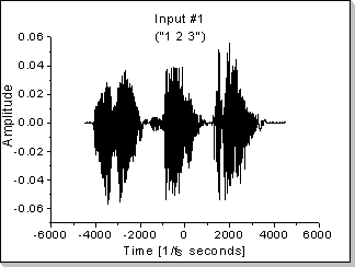 Fig.20a |
|
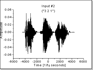 Fig.20b |
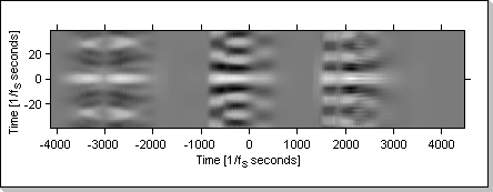
Fig.20c
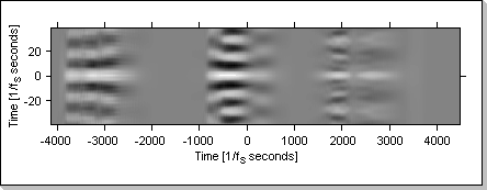
Fig.20d
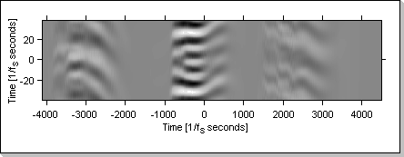
Fig.20e
Fig.20c and Fig.20d show the evolution in time of the correlation function when the same sequence is input in both the x1[] and x2[] vectors ("1 2 3" for Fig.20c and "3 2 1" for Fig.20d).
Fig.20e shows the evolution of the correlation function when the input vectors are fed with different data: x1[] is fed with the "1 2 3" sequence and x2[] is fed with the "3 2 1" sequence.
The Autocorrelation Function
A special case of correlation is the autocorrelation function; it directly results by having x2[] = x1[] (it measures the correlation between a function and its shifted replica).
Example 1
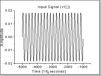 Fig.21a |
|
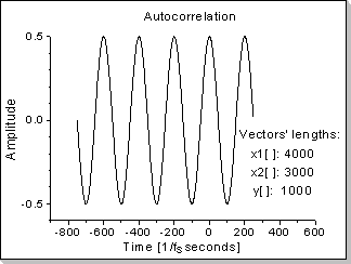 Fig.21b |
A sinus function's autocorrelation is also a sinus-shaped function (actually a cosinus, having the maximum value in zero)
Example 2
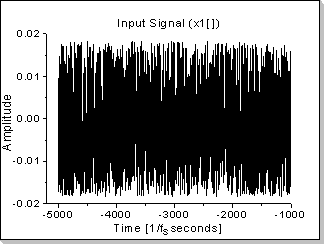 Fig.22a |
|
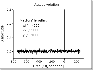 Fig.22b |
A white noise function's autocorrelation is a Dirac impulse in zero (a Kronecker0[] in the discrete domain)
Example 3
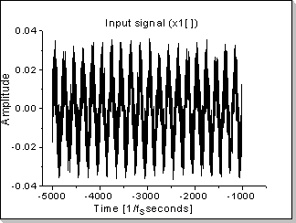 Fig.23a |
|
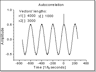 Fig.23b |
Noise filtering via autocorrelation for a noisy sinus input (having an input signal with a sinewave component and a noise component of equal amplitudes, the resulting signal will be a "cleaner" sinewave added with a Kronecker0[] impulse).